Generalized Additive Models

Generalized Additive Models

To fit a GAM in R, we could use:

1. the function gam in the mgcv package, or
2. the function gam in the gam package.

Differences between the two functions are discussed in the “Details” section of the gam documentation in the mgcv package. Choose one, but don’t load both! mgcv tends to be updated more frequently, and is generally more flexible (compare the Index pages), so that’s what is used in this tutorial. But the gam package has similar workings.

The gam function works similarly to other regression functions, but the formula specification is different. Let’s go through different formula specifications, doing regression on the mtcars dataset in R.

The formula mpg ~ disp + wt gives you a linear model. It indicates that disp and wt both enter the model in a linear fashion.

library(mgcv)

## Loading required package: nlme

## This is mgcv 1.8-31. For overview type 'help("mgcv-package")'.

fit1 <- gam(mpg ~ disp + wt, data=mtcars)
fit2 <- lm(mpg ~ disp + wt, data=mtcars)
summary(fit1)

## 
## Family: gaussian 
## Link function: identity 
## 
## Formula:
## mpg ~ disp + wt
## 
## Parametric coefficients:
##             Estimate Std. Error t value Pr(>|t|)    
## (Intercept) 34.96055    2.16454  16.151 4.91e-16 ***
## disp        -0.01773    0.00919  -1.929  0.06362 .  
## wt          -3.35082    1.16413  -2.878  0.00743 ** 
## ---
## Signif. codes:  0 '***' 0.001 '**' 0.01 '*' 0.05 '.' 0.1 ' ' 1
## 
## 
## R-sq.(adj) =  0.766   Deviance explained = 78.1%
## GCV = 9.3863  Scale est. = 8.5063    n = 32

summary(fit2)

## 
## Call:
## lm(formula = mpg ~ disp + wt, data = mtcars)
## 
## Residuals:
##     Min      1Q  Median      3Q     Max 
## -3.4087 -2.3243 -0.7683  1.7721  6.3484 
## 
## Coefficients:
##             Estimate Std. Error t value Pr(>|t|)    
## (Intercept) 34.96055    2.16454  16.151 4.91e-16 ***
## disp        -0.01773    0.00919  -1.929  0.06362 .  
## wt          -3.35082    1.16413  -2.878  0.00743 ** 
## ---
## Signif. codes:  0 '***' 0.001 '**' 0.01 '*' 0.05 '.' 0.1 ' ' 1
## 
## Residual standard error: 2.917 on 29 degrees of freedom
## Multiple R-squared:  0.7809, Adjusted R-squared:  0.7658 
## F-statistic: 51.69 on 2 and 29 DF,  p-value: 2.744e-10

Notice that the coefficient estimates are the same.

To make a term non-parametric, wrap the s function around the term (for splines; comes with the mgcv package). The gam package also has a lo function, for loess smoothing.

fit3 <- gam(mpg ~ s(disp) + s(wt), data=mtcars)
summary(fit3)

## 
## Family: gaussian 
## Link function: identity 
## 
## Formula:
## mpg ~ s(disp) + s(wt)
## 
## Parametric coefficients:
##             Estimate Std. Error t value Pr(>|t|)    
## (Intercept)  20.0906     0.3429   58.59   <2e-16 ***
## ---
## Signif. codes:  0 '***' 0.001 '**' 0.01 '*' 0.05 '.' 0.1 ' ' 1
## 
## Approximate significance of smooth terms:
##           edf Ref.df     F  p-value    
## s(disp) 6.263  7.386 6.373 0.000164 ***
## s(wt)   1.000  1.000 4.015 0.056434 .  
## ---
## Signif. codes:  0 '***' 0.001 '**' 0.01 '*' 0.05 '.' 0.1 ' ' 1
## 
## R-sq.(adj) =  0.896   Deviance explained = 92.1%
## GCV = 5.0715  Scale est. = 3.762     n = 32

Now, each predictor enters the model in a non-parametric, additive form. The nonparametric functions can be accessed by calling plot. For documentation, see ?plot.gam. Let’s plot the “bivariate” scatterplots behind these curves too (these bivariate data actually use partial residuals).

plot(fit3, residuals=TRUE)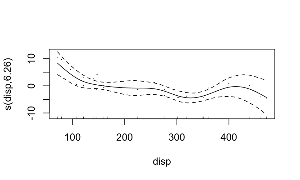

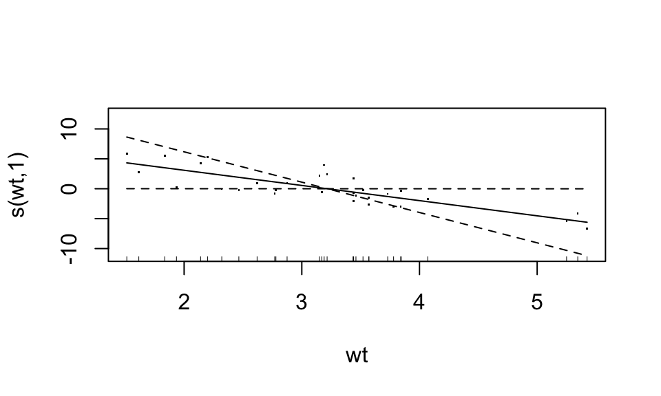
Looks like the “weight” variable (wt) is quite linear. We can let it be linear, while the disp variable remains nonparametric. “Wiggliness” of the smoothed fit can be controlled through the k argument of the s function, but this is chosen in a “smart” way by default.

fit4 <- gam(mpg ~ s(disp, k=3) + wt, data=mtcars)
summary(fit4)

## 
## Family: gaussian 
## Link function: identity 
## 
## Formula:
## mpg ~ s(disp, k = 3) + wt
## 
## Parametric coefficients:
##             Estimate Std. Error t value Pr(>|t|)    
## (Intercept)  31.1110     3.1336   9.928  1.1e-10 ***
## wt           -3.4254     0.9649  -3.550  0.00138 ** 
## ---
## Signif. codes:  0 '***' 0.001 '**' 0.01 '*' 0.05 '.' 0.1 ' ' 1
## 
## Approximate significance of smooth terms:
##          edf Ref.df     F  p-value    
## s(disp) 1.93  1.995 9.724 0.000758 ***
## ---
## Signif. codes:  0 '***' 0.001 '**' 0.01 '*' 0.05 '.' 0.1 ' ' 1
## 
## R-sq.(adj) =  0.839   Deviance explained = 85.4%
## GCV =  6.659  Scale est. = 5.8413    n = 32

plot(fit4, residuals=TRUE)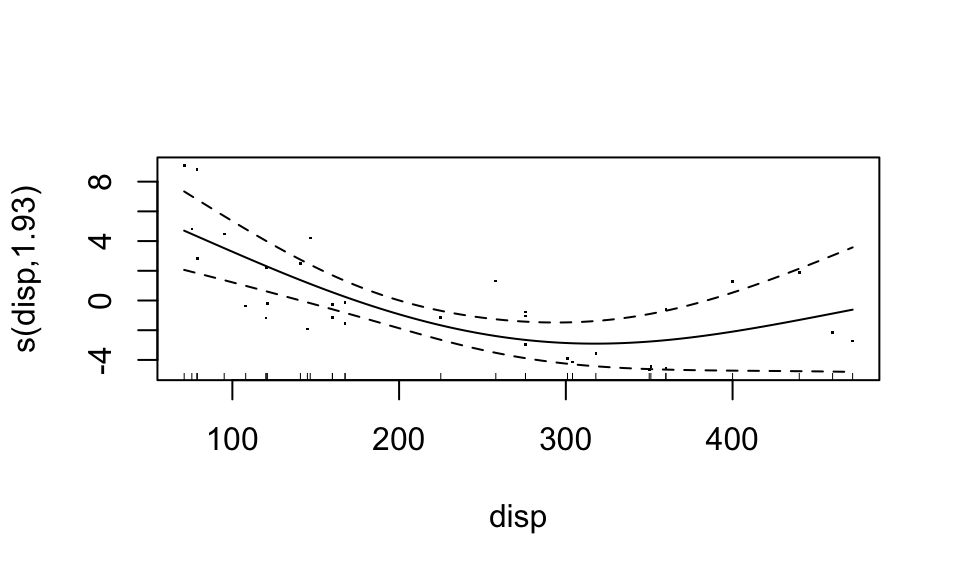

You can even combine predictors into a common smooth function:

fit5 <- gam(mpg ~ s(disp, qsec) + wt, data=mtcars)
summary(fit5)

## 
## Family: gaussian 
## Link function: identity 
## 
## Formula:
## mpg ~ s(disp, qsec) + wt
## 
## Parametric coefficients:
##             Estimate Std. Error t value Pr(>|t|)    
## (Intercept)   32.181      4.340   7.415 1.83e-07 ***
## wt            -3.758      1.345  -2.794   0.0105 *  
## ---
## Signif. codes:  0 '***' 0.001 '**' 0.01 '*' 0.05 '.' 0.1 ' ' 1
## 
## Approximate significance of smooth terms:
##                edf Ref.df     F  p-value    
## s(disp,qsec) 7.634  9.694 5.353 0.000312 ***
## ---
## Signif. codes:  0 '***' 0.001 '**' 0.01 '*' 0.05 '.' 0.1 ' ' 1
## 
## R-sq.(adj) =  0.903   Deviance explained =   93%
## GCV = 5.0335  Scale est. = 3.5181    n = 32

For each, the predict and residuals functions work in the same old way. Let’s use them to make a residual plot:

qplot(predict(fit5), residuals(fit5)) +
    geom_abline(intercept=0, slope=0, linetype="dashed") +
    xlab("Prediction (mean)") + ylab("Residuals")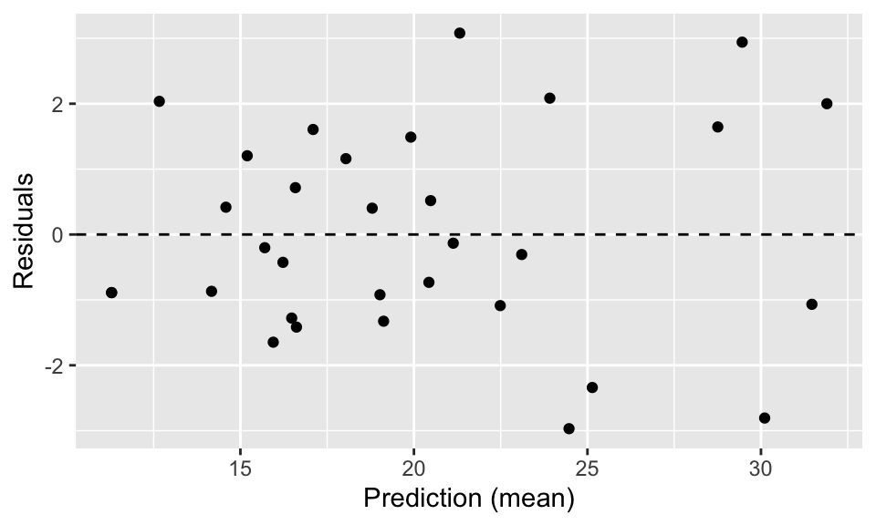

For their documentation, see ?predict.gam and ?residuals.gam.