JAGS Tutorial

JAGS is a language that allows you to run Bayesian analyses. It gets at the posterior by generating samples based on the posterior and statistical model.

You’ll need to download and install JAGS. You can interact with JAGS through one of three R packages:

• runjags (recommended for this course)
  • Model written as a single string in R; possibly also allows you to input from file.
  • Quick-start guide vignette: vignette("quickjags", package="runjags")
  • Full user guide vignette: vignette("UserGuide", package="runjags")
• rjags (sample code here)
  • Model read in from plain text file.
• R2jags
  • this is dependent on R2winbugs, which I find doesn’t work well outside of Windows machines, so I’m more hesitant to use this package.
  • Model written in R as a function, but using JAGS language; or inputted from file.

Also, the coda package is useful for working with the output of at least runjags.

About the JAGS language:

• Generates samples of parameters based on the prior and statistical model.
• Need to specify which parameters you want to include in the output (aka “track” or “monitor”).
• Specify probability distributions similarly to R, except:
  • Draw samples using calls like dexp and dnorm, not rexp and rnorm.
  • The JAGS version of rnorm uses the precision (=1/variance) instead of standard deviation. The documentation of JAGS code is not as nice as R. You have to look things up from a table-of-contents-style search from this document. Page 29 shows the aliases for various distributions.

For this week’s lab assignment (3), you’ll only be using it to generate observations from a distribution. Let’s generate data from a N(0,2) distribution (that is, variance=2), and ignore the warning messages for this week.

library(runjags)
my_model <- "
model{
    # This is a comment.
    theta ~ dnorm(0, 1/2)
}
"
fit <- run.jags(my_model, monitor = "theta", n.chains = 1, sample = 1000)

## Calling the simulation...
## Welcome to JAGS 4.3.0 on Thu Sep 30 22:16:26 2021
## JAGS is free software and comes with ABSOLUTELY NO WARRANTY
## Loading module: basemod: ok
## Loading module: bugs: ok
## . . Compiling model graph
##    Resolving undeclared variables
##    Allocating nodes
## Graph information:
##    Observed stochastic nodes: 0
##    Unobserved stochastic nodes: 1
##    Total graph size: 5
## . Initializing model
## . Adaptation skipped: model is not in adaptive mode.
## . Updating 4000
## -------------------------------------------------| 4000
## ************************************************** 100%
## . . Updating 1000
## -------------------------------------------------| 1000
## ************************************************** 100%
## . . . . Updating 0
## . Deleting model
## . 
## Note: the model did not require adaptation
## Simulation complete.  Reading coda files...
## Coda files loaded successfully
## Calculating summary statistics...
## Finished running the simulation

theta <- coda::as.mcmc(fit)
head(theta)

## Markov Chain Monte Carlo (MCMC) output:
## Start = 5001 
## End = 5007 
## Thinning interval = 1 
##           theta
## 5001  1.2975400
## 5002  0.7812320
## 5003  0.7415140
## 5004  2.0970800
## 5005 -0.0261437
## 5006 -2.1801300
## 5007 -0.9571290

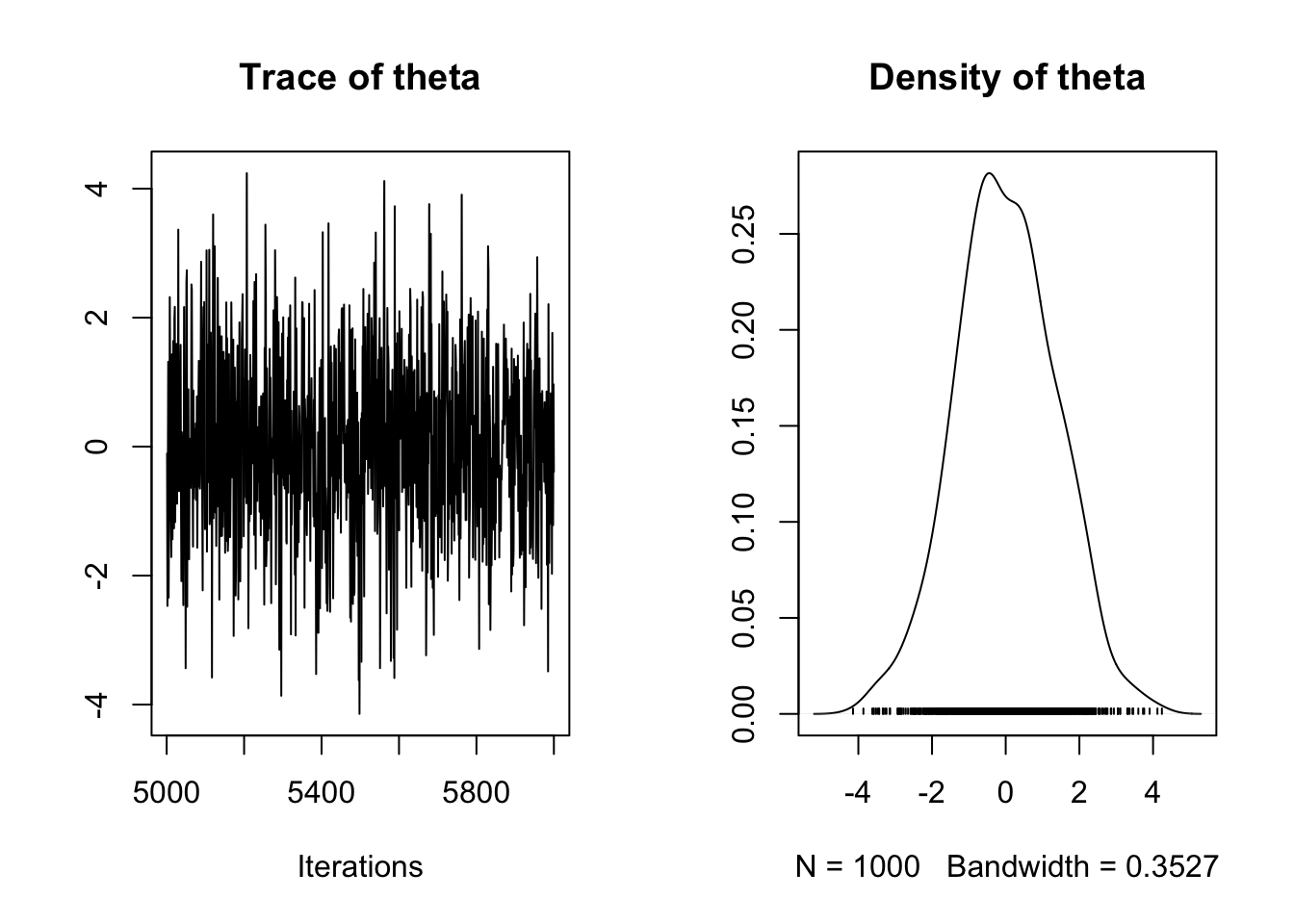
plot(theta)

library(tidyverse)

## ── Attaching packages ─────────────────────────────────────── tidyverse 1.3.0 ──

## ✓ ggplot2 3.3.2     ✓ purrr   0.3.4
## ✓ tibble  3.0.3     ✓ dplyr   1.0.2
## ✓ tidyr   1.1.2     ✓ stringr 1.4.0
## ✓ readr   1.3.1     ✓ forcats 0.5.0

## ── Conflicts ────────────────────────────────────────── tidyverse_conflicts() ──
## x tidyr::extract() masks runjags::extract()
## x dplyr::filter()  masks stats::filter()
## x dplyr::lag()     masks stats::lag()

library(runjags)
n <- 50
dat <- tibble(x = rnorm(n),
              y = x + rnorm(n))
jagsdat <- c(as.list(dat), n = nrow(dat))
model <- "model{
    for (i in 1:n) {
        y[i] ~ dnorm(beta*x[i], tau)
    }
    tau <- pow(sigma, -2)
    sigma ~ dunif(0, 100)
    beta ~ dnorm(0, 0.001)
}"
foo <- run.jags(
    model = model, 
    monitor = c("beta0", "beta1", "sigma"), 
    data = jagsdat
)

## Warning: No initial value blocks found and n.chains not specified: 2 chains were
## used

## Warning: No initial values were provided - JAGS will use the same initial values
## for all chains

## Calling the simulation...
## Welcome to JAGS 4.3.0 on Thu Sep 30 22:16:29 2021
## JAGS is free software and comes with ABSOLUTELY NO WARRANTY
## Loading module: basemod: ok
## Loading module: bugs: ok
## . . Reading data file data.txt
## . Compiling model graph
##    Resolving undeclared variables
##    Allocating nodes
## Graph information:
##    Observed stochastic nodes: 50
##    Unobserved stochastic nodes: 2
##    Total graph size: 159
## . Initializing model
## . Adapting 1000
## -------------------------------------------------| 1000
## ++++++++++++++++++++++++++++++++++++++++++++++++++ 100%
## Adaptation successful
## . Updating 4000
## -------------------------------------------------| 4000
## ************************************************** 100%
## . Failed to set trace monitor for beta0
## Variable beta0 not found
## . Failed to set trace monitor for beta1
## Variable beta1 not found
## . . Updating 10000
## -------------------------------------------------| 10000
## ************************************************** 100%
## . . . . . Updating 0
## . Deleting model
## . 
## Simulation complete.  Reading coda files...
## Coda files loaded successfully
## Calculating summary statistics...
## Calculating the Gelman-Rubin statistic for 1 variables....
## Finished running the simulation

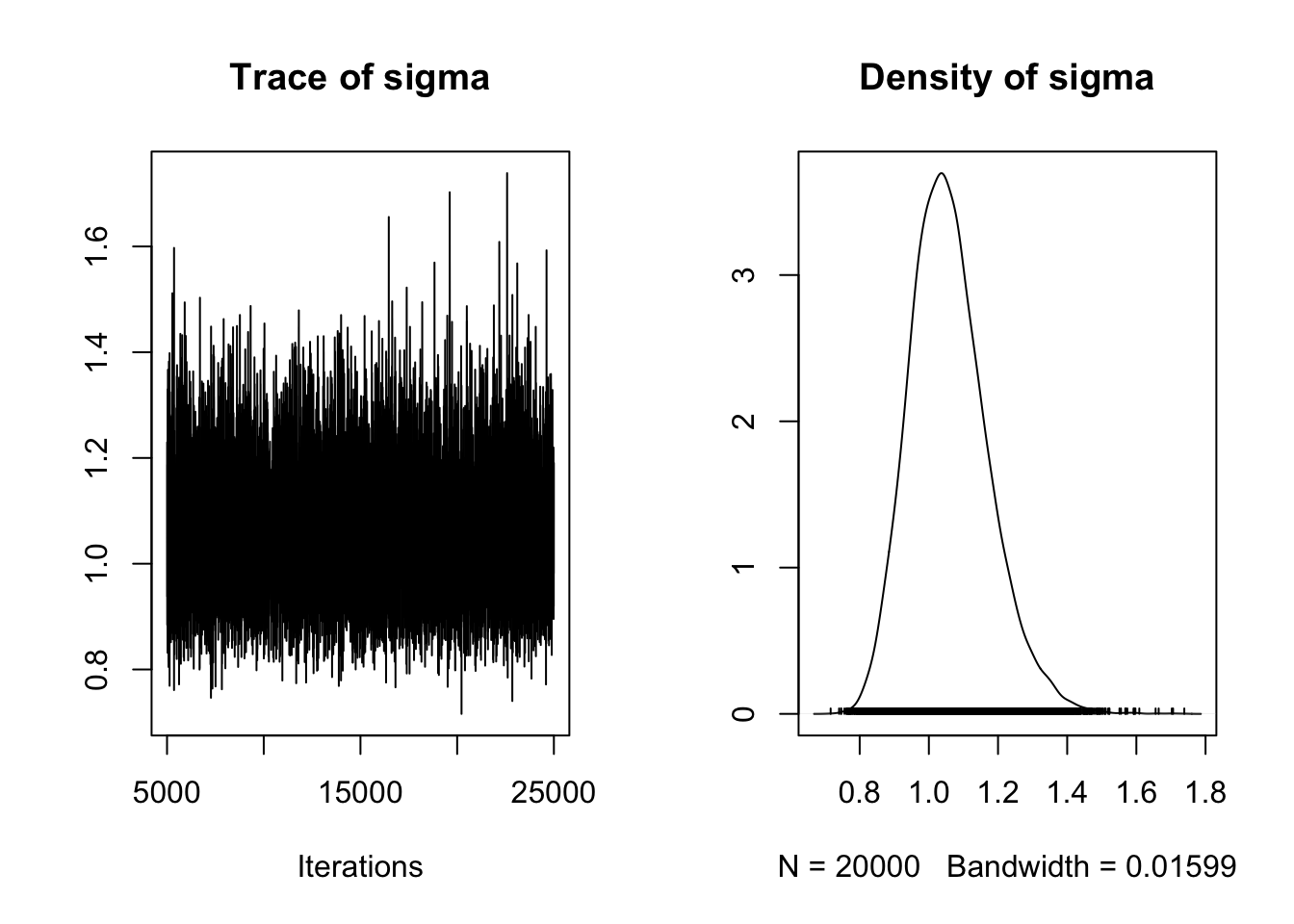
plot(coda::as.mcmc(foo))

## Warning in as.mcmc.runjags(foo): Combining the 2 mcmc chains together